How To Draw On Excel Graph

Once you input your data and select the cell range, you're ready to choose your chart type to brandish your data. In this case, we'll create a clustered column nautical chart from the information we used in the previous section.

Pace 1: Select Chart Type

Once your data is highlighted in the Workbook, click the Insert tab on the meridian banner. Nearly halfway across the toolbar is a section with several chart options. Excel provides Recommended Charts based on popularity, but you can click any of the dropdown menus to select a unlike template.

Step two: Create Your Nautical chart

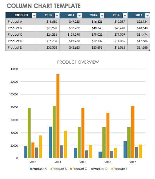
1. From the Insert tab, click the cavalcade chart icon and select Clustered Column.

​

1. Excel volition automatically create a clustered chart column from your selected information. The chart will appear in the center of your workbook.
2. To name your chart, double click the Nautical chart Title text in the chart and type a title. We'll call this nautical chart "Product Turn a profit 2022 - 2022."

​

We'll utilise this chart for the balance of the walkthrough. You can download this same nautical chart to follow along.

Download Sample Column Nautical chart Template

There are two tabs on the toolbar that you lot will utilize to brand adjustments to your chart: Chart Blueprint and Format. Excel automatically applies design, layout, and format presets to charts and graphs, but you tin can add together customization by exploring the tabs. Next, we'll walk you through all the bachelor adjustments in Chart Design.

Step 3: Add together Chart Elements

Adding chart elements to your nautical chart or graph will heighten information technology by clarifying information or providing additional context. You can select a chart element past clicking on the Add Chart Element dropdown card in the top left-paw corner (beneath the Home tab).

To Display or Hide Axes:

1. Select Axes. Excel will automatically pull the column and row headers from your selected cell range to display both horizontal and vertical axes on your chart (Nether Axes, there is a check mark next to Primary Horizontal and Chief Vertical.)

   

2. Uncheck these options to remove the brandish axis on your nautical chart. In this example, clicking Main Horizontal will remove the twelvemonth labels on the horizontal axis of your chart.

   

3. Click More Axis Options… from the Axes dropdown menu to open a window with additional formatting and text options such as adding tick marks, labels, or numbers, or to change text color and size.

   

To Add together Axis Titles:

1. Click Add Chart Element and click Axis Titles from the dropdown menu. Excel will not automatically add axis titles to your nautical chart; therefore, both Principal Horizontal and Primary Vertical will be unchecked.

   

2. To create axis titles, click Primary Horizontal or Master Vertical and a text box will appear on the chart. We clicked both in this example. Type your centrality titles. In this example, the nosotros added the titles "Year" (horizontal) and "Profit" (vertical).

   

To Remove or Move Chart Title:

• Click Add together Nautical chart Chemical element and click Chart Championship. You volition see four options: None, Above Chart, Centered Overlay, and More than Title Options.

  

• Click None to remove chart championship.
• Click Above Chart to place the championship above the nautical chart. If you create a chart title, Excel will automatically identify it above the chart.
• Click Centered Overlay to place the title within the gridlines of the chart. Exist careful with this option: you don't want the title to cover any of your information or clutter your graph (as in the example below).

To Add Data Labels:

1. Click Add Chart Element and click Data Labels. There are half-dozen options for data labels: None (default), Center, Within End, Inside Base, Outside Cease, and More Data Label Championship Options.

   

2. The 4 placement options will add specific labels to each data bespeak measured in your chart. Click the option you desire. This customization can exist helpful if you have a small amount of precise data, or if you take a lot of extra infinite in your chart. For a amassed cavalcade nautical chart, withal, adding data labels will likely look too cluttered. For example, hither is what selecting Center information labels looks like:

   

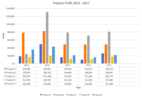
To Add together a Data Table:

1. Click Add Chart Element and click Data Table. There are iii pre-formatted options along with an extended carte du jour that can exist plant by clicking More Data Table Options:

   

• None is the default setting, where the information table is non duplicated inside the nautical chart.
• With Fable Keys displays the data table below the chart to evidence the data range. The color-coded fable will also be included.

  

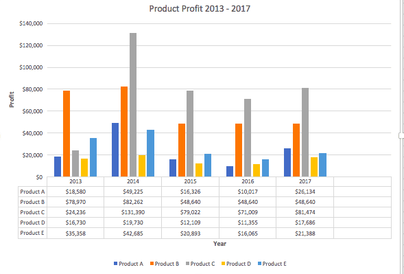
• No Legend Keys also displays the data table beneath the chart, only without the legend.

  

Note: If you choose to include a data tabular array, yous'll probably want to brand your chart larger to accommodate the table. Merely click the corner of your chart and use elevate-and-driblet to resize your chart.

To Add Error Bars:

1. Click Add Chart Chemical element and click Error Bars. In addition to More Error Bars Options, in that location are four options: None (default), Standard Error, 5% (Pct), and Standard Deviation. Adding fault bars provide a visual representation of the potential error in the shown data, based on different standard equations for isolating mistake.

   

2. For example, when nosotros click Standard Error from the options nosotros get a chart that looks similar the image below.

   

 To Add Gridlines:

1. Click Add together Nautical chart Element and click Gridlines. In add-on to More than Grid Line Options, there are four options: Main Major Horizontal, Principal Major Vertical, Primary Minor Horizontal, and Primary Pocket-size Vertical. For a cavalcade chart, Excel volition add Main Major Horizontal gridlines by default.

   

2. You can select every bit many different gridlines as you want past clicking the options. For example, here is what our chart looks like when we click all four gridline options.

   

To Add a Legend:

1. Click Add Chart Element and click Legend. In addition to More Legend Options, in that location are five options for fable placement: None, Correct, Pinnacle, Left, and Bottom.

   

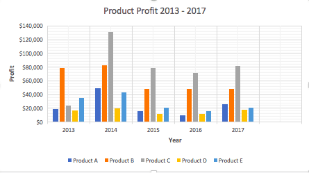
2. Fable placement will depend on the style and format of your chart. Check the choice that looks all-time on your nautical chart. Here is our chart when we click the Right legend placement.

   

To Add Lines: Lines are not bachelor for amassed column charts. All the same, in other chart types where you lot only compare ii variables, you can add lines (east.g. target, average, reference, etc.) to your nautical chart by checking the appropriate pick.

To Add a Trendline:

1. Click Add Nautical chart Chemical element and click Trendline. In improver to More Trendline Options, at that place are v options: None (default), Linear, Exponential, Linear Forecast, and Moving Average. Cheque the appropriate pick for your information set. In this instance, nosotros volition click Linear.

   

2. Because nosotros are comparison five different products over fourth dimension, Excel creates a trendline for each individual product. To create a linear trendline for Product A, click Product A and click the bluish OK button.

   

3. The chart will at present display a dotted trendline to stand for the linear progression of Product A. Note that Excel has besides added Linear (Product A) to the fable.

   

4. To brandish the trendline equation on your chart, double click the trendline. A Format Trendline window will open up on the right side of your screen. Click the box adjacent to Brandish equation on nautical chart at the bottom of the window. The equation now appears on your nautical chart.

   

Notation: You can create carve up trendlines for every bit many variables in your nautical chart equally you similar. For example, hither is our chart with trendlines for Product A and Product C.

To Add Upward/Down Bars: Upward/Down Confined are non available for a cavalcade chart, simply you can use them in a line chart to show increases and decreases among data points.

Step 4: Suit Quick Layout

1. The 2d dropdown bill of fare on the toolbar is Quick Layout, which allows you to quickly alter the layout of elements in your chart (titles, legend, clusters etc.).

   

2. There are 11 quick layout options. Hover your cursor over the unlike options for an explanation and click the one you desire to apply.

   

Pace 5: Change Colors

The next dropdown menu in the toolbar is Alter Colors. Click the icon and choose the colour palette that fits your needs (these needs could be aesthetic, or to lucifer your brand'south colors and fashion).

Step 6: Alter Way

For cluster cavalcade charts, there are 14 chart styles available. Excel will default to Manner one, but you lot can select any of the other styles to change the nautical chart appearance. Use the arrow on the right of the epitome bar to view other options.

Step 7: Switch Row/Column

1. Click the Switch Row/Column on the toolbar to flip the axes. Note: It is not e'er intuitive to flip axes for every chart, for example, if you take more than than 2 variables.

   

In this example, switching the row and cavalcade swaps the production and year (profit remains on the y-axis). The chart is at present clustered by production (not twelvemonth), and the color-coded legend refers to the yr (non production). To avert defoliation here, click on the legend and change the titles from Series to Years.

Step eight: Select Data

1. Click the Select Data icon on the toolbar to change the range of your data.

   

2. A window volition open up. Type the prison cell range you want and click the OK button. The chart will automatically update to reflect this new data range.

   

Footstep 9: Change Chart Blazon

1. Click the Modify Chart Type dropdown menu.

   

2. Hither you can change your nautical chart type to any of the nine chart categories that Excel offers. Of class, brand sure that your data is appropriate for the nautical chart type yous choose.

   

3. Y'all can also salvage your nautical chart as a template by clicking Save as Template…

4. A dialogue box will open where y'all can proper noun your template. Excel volition automatically create a folder for your templates for easy system. Click the blue Save button.

   

Step 10: Motion Chart

1. Click the Motion Chart icon on the far right of the toolbar.

   

2. A dialogue box appears where you can cull where to place your chart. You can either create a new sheet with this nautical chart (New sheet) or place this chart as an object in another canvas (Object in). Click the blueish OK button.

   

Step 11: Change Formatting

1. The Format tab allows y'all to change formatting of all elements and text in the chart, including colors, size, shape, fill, and alignment, and the ability to insert shapes. Click the Format tab and use the shortcuts available to create a chart that reflects your organization'south make (colors, images, etc.).

   

2. Click the dropdown menu on the summit left side of the toolbar and click the nautical chart element y'all are editing.

   

Step 12: Delete a Nautical chart

To delete a chart, simply click on it and click the Delete key on your keyboard.

Source: https://www.smartsheet.com/how-to-make-charts-in-excel

Posted by: williamswasioneating.blogspot.com

Share this post